
Introduction of RNN
What is the RNN?
Squashing the ANN! → 요소들은 다 있지만 단지 ANN을 아래에서 보는 거라고 생각하면 이것이 RNN이다. (차원을 추가하고, 새로운 차원에서 바라보는 것)
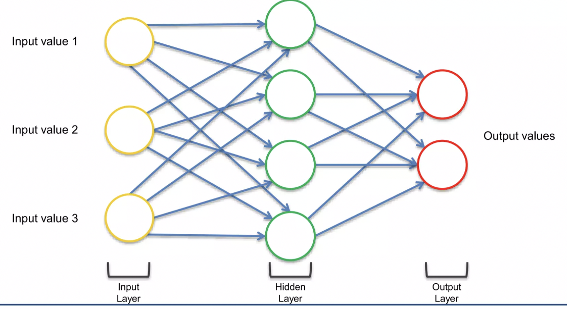
hidden layer에 해당하는 초록원을 파란색으로 바꾸고, temporal loop를 뜻하는 파란 줄을 추가해 준다. hidden layer는 output layer에 출력을 전달할 뿐만 아니라, 그 자체로도 피드백을 제공한다는 의미이다.
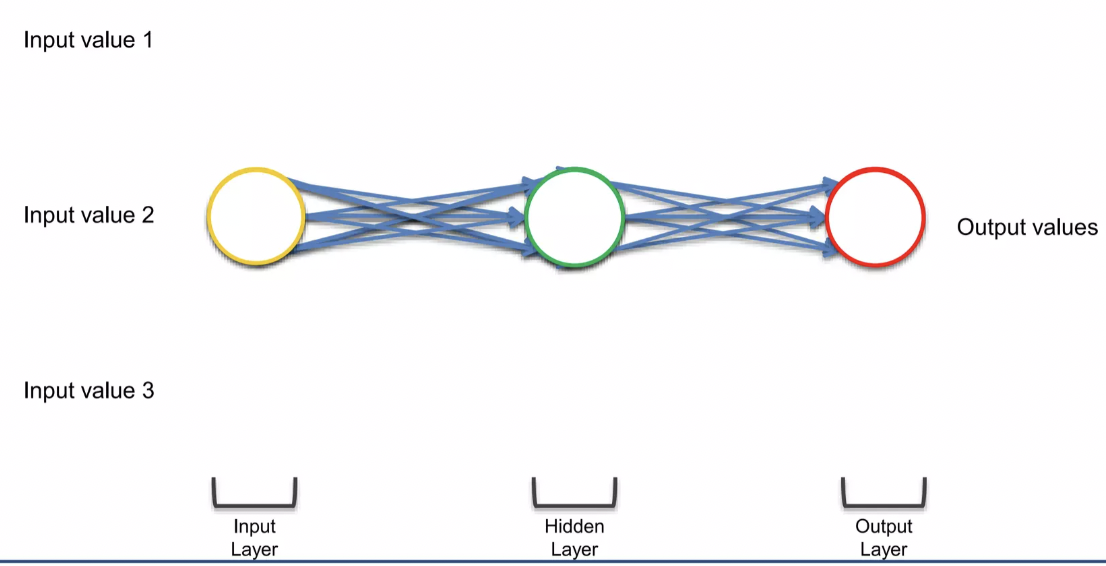
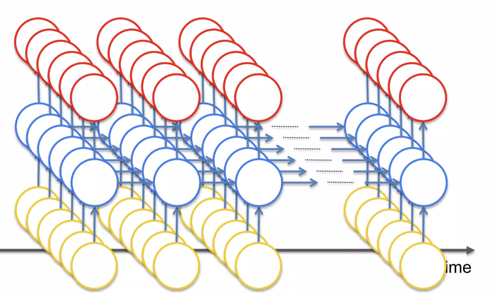
새로운 차원에서 바라보고 있지만, 결국 매우 많은 값들이 존재하고 있는 것 (→ 각각의 동그라미들은 neuron이 아니라 layer이기 때문에)
neuron으로 input이 들어오고 output이 나가는데, 시간이 지나면서 neuron들은 서로 연결된다. 이것이 바로 short-term memory 이다. (previous neuron에 뭐가 있었는지 기억하는 것!)
Examples of RNN Application
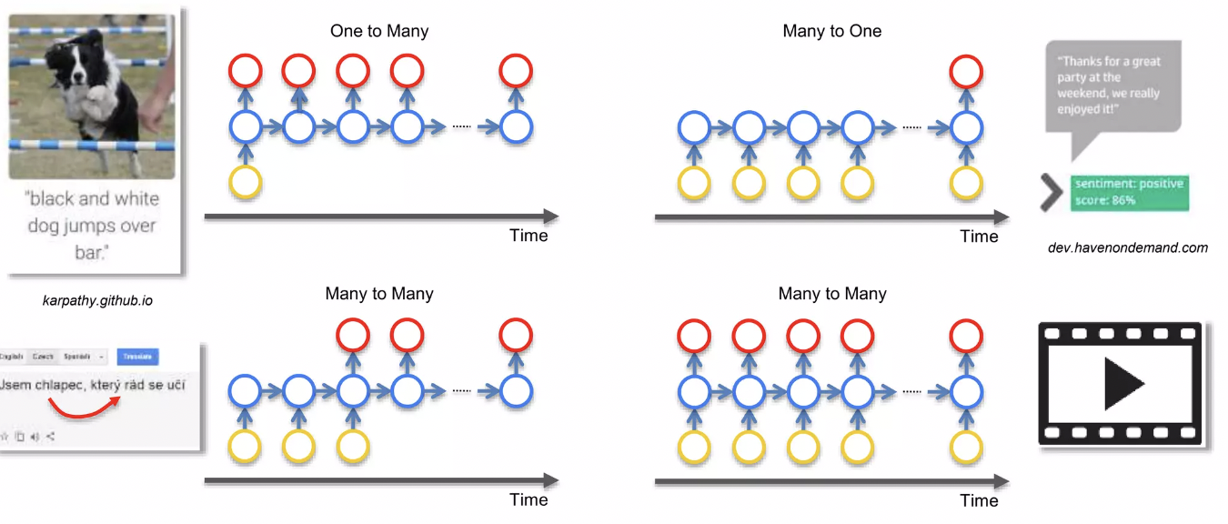
[One to many]
- 컴퓨터가 이미지를 설명하는 경우
- input이 CNN → RNN 순서로 들어가서, output으로 image를 설명하는 문장이 출력
- CNN은 image processing, feature recognition → RNN은 컴퓨터가 문장이 말이 되도록 만들어주는 기능을 수행한다.
[Many to one]
- Sentiment Analysis → text가 얼마나 positive or negative한지 알려준다.
[Many to many]
- Translations → 다음 단어를 번역하기 위해서 previous word에 관한 short-term information이 필요한데, RNN의 short-term memory로 이런 기능을 수행
- Generating subtitles for movies → 자막을 생성하려면 이전의 영화 화면(이전 내용, 맥락)의 정보가 필요하므로, CNN만으로는 수행할 수 없고, RNN의 short-term memory가 있어야한다.
Vanishing Gradient Problem
Gradient Descent Algorithm
Find global minimum of cost function (→ optimal solution, optimal set-up for the neural network)
정보가 네트워크를 통해 이동할 때, 시간과 이전 시점의 정보를 통해 이동해서 네트워크를 통해 정보를 계속 전달한다. 각 노드는 단순한 노드가 아니라 노드의 layer를 대표한다. ( → each neuron represents the layer)
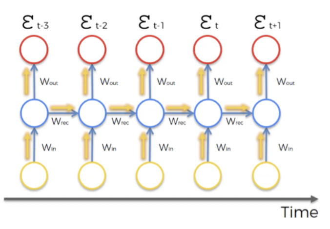
- cost function은 output value를 빨간 원안에 있는, 목표하는 output value와 비교해 준다. ( → this happens during the training, you have these values throughout the time-series)
- 즉, 각각의 붉은 원 안에서 cost function을 계산한다.
- 이 때, 해당 neuron 이 거쳐온 모든 네트워크의 neuron들의 weights들을 모두 Update한다. (50단계를 거쳐서 해당 neuron에 도달했다면, 50단계의 weights를 모두 update!)
- Wrec : 가중치 순환 → hidden layer를 펼쳐진 time loop에서 스스로에게 연결하는데 사용하는 weights를 말한다. 즉, 한 layer에서 다음 layer로 가기 위해서 값을 곱하는 것이다. 출력값에 weight를 곱하고 다음 layer로 이동하게 된다. 단, time loop를 통과할 때가지 똑같은 weights로 계속해서 곱한다.
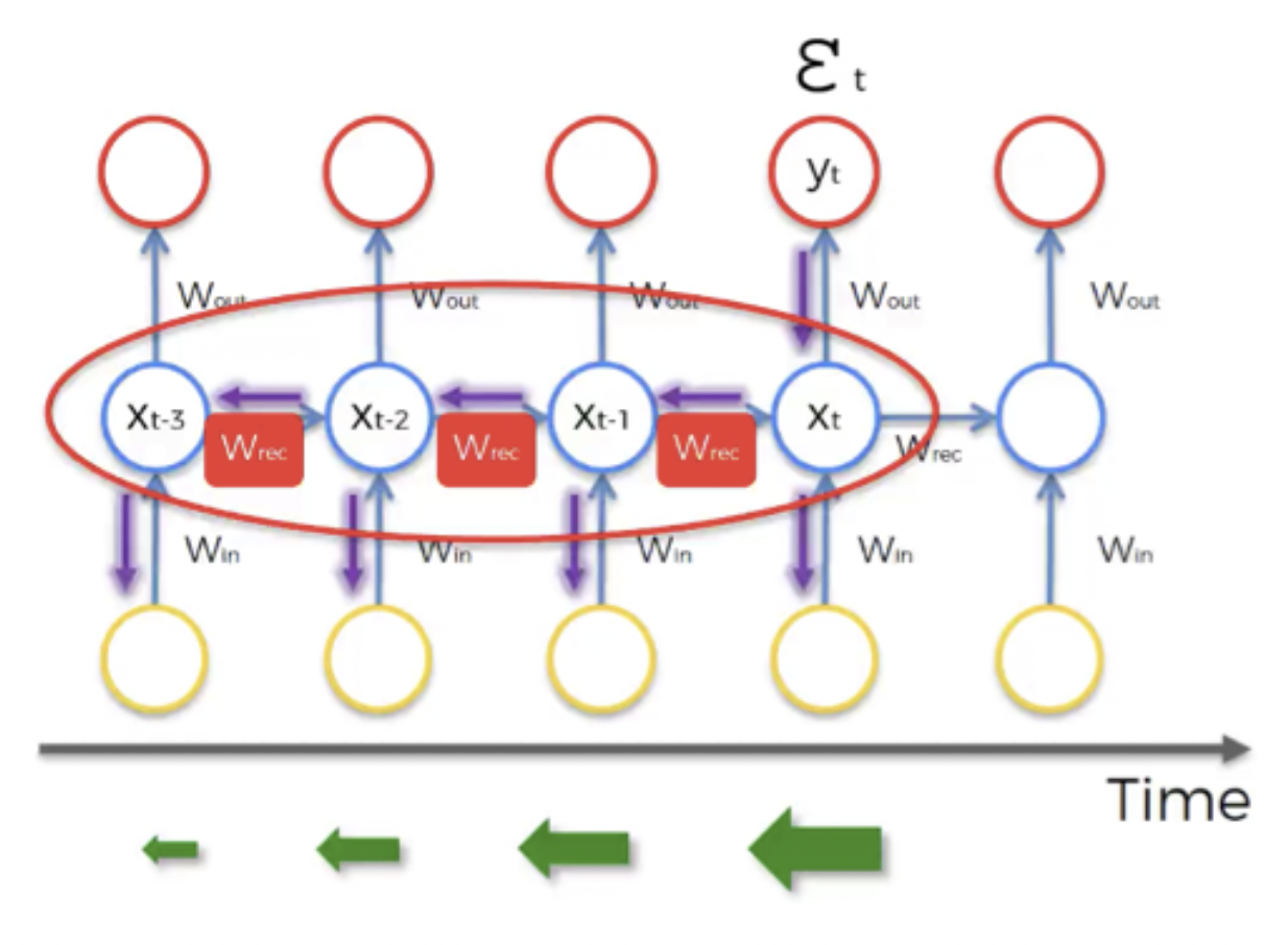
- weights는 neural network 가 시작되는 부분에서 할당되며, 이 때 0에 가까운 임의의 값으로 weights가 설정된다. 하지만 weights를 계속 여러 번 곱하게 되면 값은 매우 작아지게 되므로, 기울기가 점점 더 줄어들게 되면서 Vanishing Gradient Problem 이 발생한다.
why is vanishing gradient bad for networks?
gradient가 network를 되돌아가면서 weights를 업데이트 하는데, lower gradient이면 network가 weights를 업데이트하기 힘들어진다. 즉, gradient가 작아질수록 weights 업데이트 속도가 매우 느려진다. (gradient가 커지면 weights update 속도 빨라짐!)
또한 network의 어느 부분은 훈련받고 어느 부분은 훈련받지 않게 된다. 이 경우에 제대로 훈련받지 않은 layer의 output value가 다음 layer의 input으로 사용된다는 문제가 발생한다. 즉, 훈련이 느리게 진행될 뿐만 아니라 전달하는 output이 틀린 value를 전달하기 때문에 제대로 결과를 낼 수 없는 network를 만들어 낸다. ( → domino effect, 악순환 발생!)
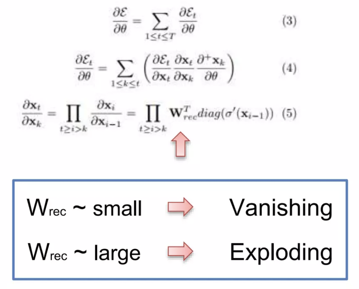
- Wrec이 작으면 → vanishing gradient problem 발생!
- Wrec이 크면 → exploding gradient problem 발생!
What are the Solutions to these problems?
[Exploding Gradient]
- Truncated Backpropagation : 특정 시점이 지나면 backpropagation을 멈춤. (하지만 모든 weights를 업데이트하지 못하기 때문에 optimal solution은 아님)
- Penalties : gradient가 penalties를 받고 인위적으로 감소한다.
- Gradient Clipping : gradient의 maximum value를 설정한다.
[Vanishing Gradient]
- Weight Initialization : vanishing gradient problem의 가능성을 최소화하기 위해서 가중치를 초기화하는 것
- Long Short-Term Memory Networks(LSTMs)
LSTMs (Long Short-Term Memory Networks)
Structure of LSTM
Wrec 이 1보다 작다면 vanishing gradient problem이 생기고, Wrec 이 1보다 크다면 exploding gradient problem이 생긴다.
⇒ Wrec = 1 이라면 모든 문제가 해결! 이것이 LSTM에서 하는일
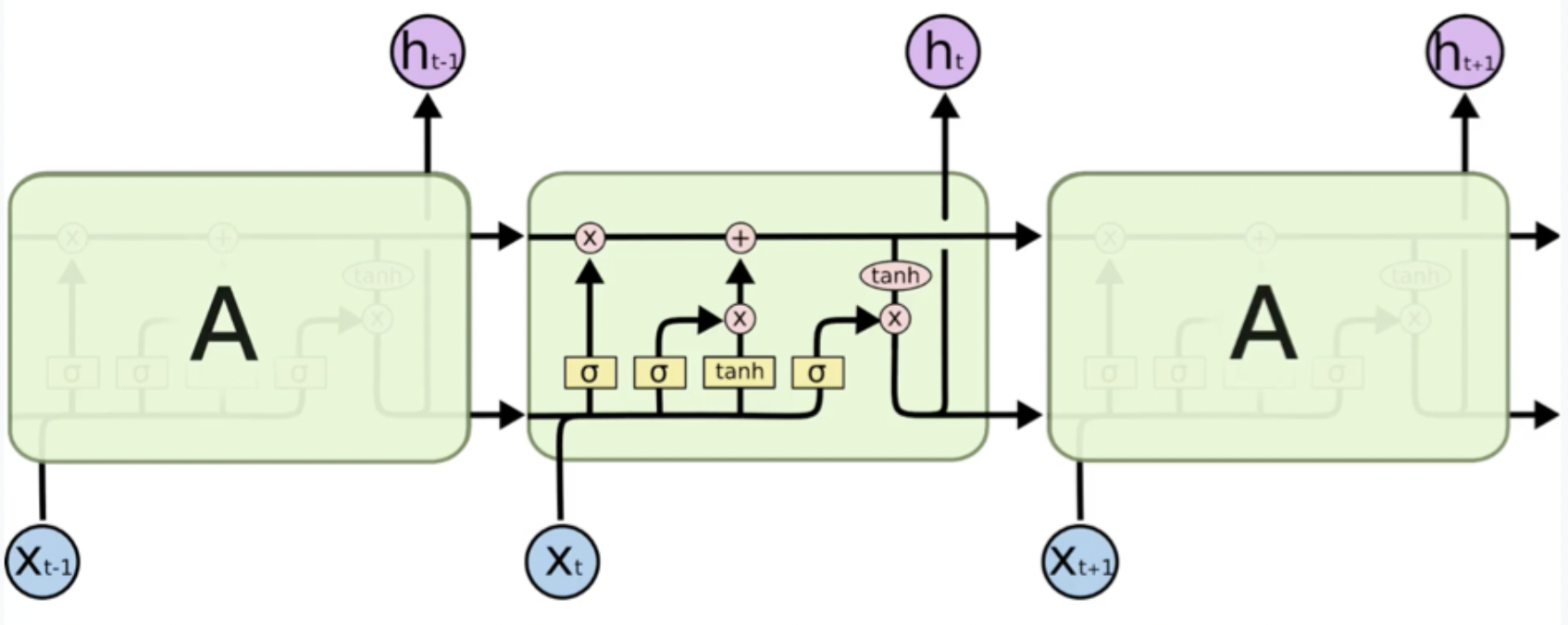
- Wrec : 맨 위의 줄 (2 point-wise operation 존재!)
- Memory cell(memory pipeline): 자유롭게 시간을 통과하면서, 제거/추가 될 수 있다. 시간을 자유롭게 이동하기 때문에, LSTM을 통해서 back-propagation하면 vanishing gradient problem이 발생하지 않는다.
Notation
- ct-1 : stands for the input from a memory cell in time point t
- xt : is an input in time point t
- ht : is an output in time point t that goes to both the output layer and the hidden layer in the next time point.
- 모든 값들은 단일의 값이 아니라, 매우 많은 값들로 이루어진 vector로 존재한다. ( → neuron이 아니라 layer이기 때문!)
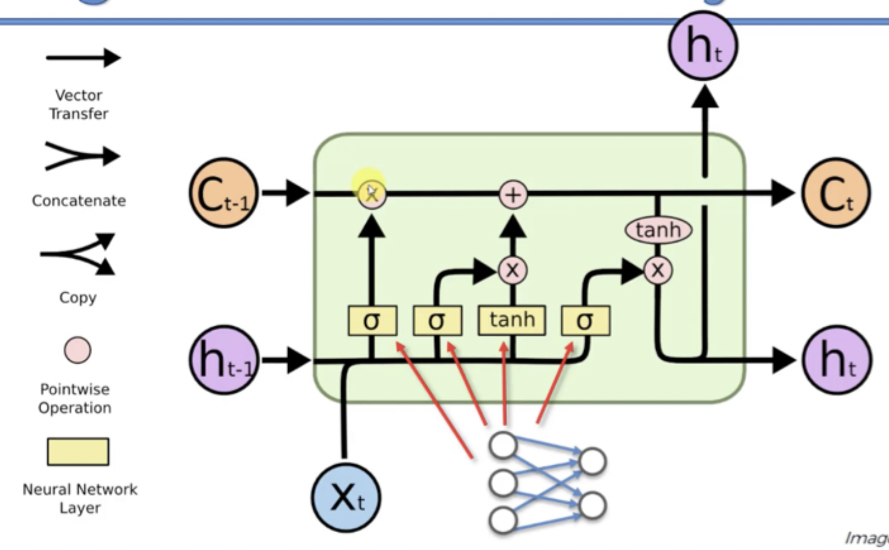
LSTM architecture step by step
- We’ve got new value xt and value from the previous node ht-1 coming in.
- These values are combined together and go through the sigmoid activation function, where it is decided if the forget valve should be open, closed or open to some extent. (밸브를 열지말지 생각!)
- The same values, or actually vectors of values, go in parallel through another layer operation “tanh” (→ 결합되는 것은 아님!), where it is decided what value we’re going to pass to the memory pipeline, and also sigmoid layer operation, where it is decided, if that value is going to be passed to the memory pipeline and to what extent.
- Then, we have a memory flowing through the top pipeline( → Wrec 줄을 말하는 것). If we have forget valve open and memory valve closed then the memory will not change. Otherwise, if we have forget valve closed and memory valve open, the memory will be updated completely.
- Finally, we’ve got xt and ht-1 combined to decide what part of the memory pipeline is going to become the output of this module.

